

d = ∑ln(1 + |Bi - Ai|)which has been dubbed the Lorentzian [Cha, 2007]. It is not indicated which Lorentz it is named after!

Software package GOPAK uses an expanded concept of orthogonality to give alternative solutions to
standard problems in linear algebra. While the concepts of generalized orthogonality have been known to mathematics
for many years, GOPAK appears to be the first program to actually compute such vectors.
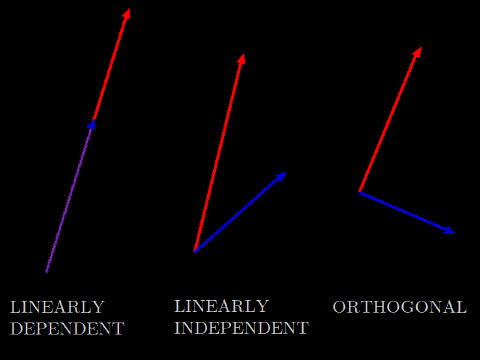
A common task in linear algebra is to ask, given a set of vectors, if one of the set can be represented as a linear combination of the others. If so, then the set is linearly dependent. If not, the set is linearly independent. In the plane, linearly dependent vectors are collinear, and linearly independent vectors meet at an angle other than 0° or 180°. The purest form of linear independence occurs when no vector contains any component of any other. Such a set is called orthogonal.
An application of orthogonality is linear regression. Suppose you want to predict something, for example, the share
price of Ford Motor Company after one year. Suppose there is some data on which to base a prediction, for example, the
entries on the company's quarterly balance sheet. Suppose further that a satisfactory prediction can be made as a
linear combination of these values, and that some data is available that relates past balance sheet entries to changes
in share price. Multiple linear regression finds factors βj so that the linear combination
yi ≈ ŷi = ∑Xijβjis an estimate of the value to be predicted.
Suppose an adequate amount of information has been collected on corporate balance-sheet entries and share price changes. Arrange the balance-sheet information into matrix X and the price changes into vector y, something like:
| Inventory | Property, plant & equipment | Accounts payable | |
|---|---|---|---|
| Ford | x11 | x12 | x13 |
| Visa | x21 | x22 | x23 |
| Pfizer | x31 | x32 | x33 |
| Goldman Sachs | x41 | x42 | x43 |
| DowDuPont | x51 | x52 | x53 |
| Change in share price | |
|---|---|
| Ford | y1 |
| Visa | y2 |
| Pfizer | y3 |
| Goldman Sachs | y4 |
| DowDuPont | y5 |
(ŷ - y) ⊥ Xβand so orthogonality is the key to solving multiple regression problems.
When m < n, the problem is underdetermined. There is an infinity of ways to choose β to satisfy y = Xβ. One approach is to choose β so as to give weight to the columns of X that are most nearly aligned to y. Since parallelism is the opposite of orthogonality, the method of assessing orthogonality can also be used to choose the columns most parallel to y. Thus, orthogonality is also the key to solving the underdetermined problem.
It is possible for a system of linear equations to be both overdetermined and underdetermined, because of linear dependence between the rows or columns.
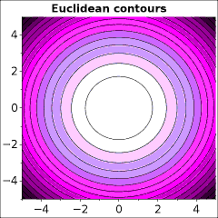
Mathematicians who research non-Euclidean geometry take the approach of discarding some axiom and exploring the consequences. The present article will take the opposite position: that it is obligatory to explain beforehand what justification exists for neglecting any property of Euclidean space.

The Pythagorean theorem can be proved simply by taking four tiles, each a right triangle with sides AxB, and rearranging them inside a square with an edge of A+B. Measuring the remaining area, A² + B² = C². How could this ever be wrong?
First, drawing a plot of one variable against another can be misleading. For example, plotting a curve of temperature against pressure renders these quantities into geometry. This is only an analogy! You can't add apples and oranges, and you can't add squared temperature to squared pressure. Distances on such a plot are without physical meaning.
Second, the condition that the prediction error be orthogonal to the prediction is equivalent to the condition that the sum of the individual squared errors be minimized. (See appendix.) This means, for example, minimizing an error measured in squared dollars. This quantity has no business significance; it would make more sense to minimize the total absolute values of prediction error, a quantity measured in dollars.
Keeping this justification in mind, alternative definitions of orthogonality may be considered in geometries in which the Pythagorean theorem does not apply.
d = (∑(Bj - Aj)p)1/pwhere p > 0. When p = 2, this reduces to the Pythagorean theorem. Other values of p yield different distance functions and a well-studied family of non-Euclidean geometries.
The isosceles orthogonality criterion [Roberts, 1934] says that two vectors u and v are orthogonal if and only if the distance from u to v is the same as the distance from u to negative v.
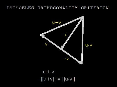
When distance is given by the Pythagorean theorem, the isosceles criterion is equivalent to Euclidean orthogonality. Other distance functions give different meanings to orthogonal. Isosceles orthogonality is symmetric, so that u ⊥ v ⇔ v ⊥ u
A residual orthogonality criterion [Birkhoff, 1935] says that vectors u and v are orthogonal when no multiple of u can be added to v such that the sum v + su has a magnitude less than v. When distance is given by the Pythagorean theorem, the residual criterion is equivalent to Euclidean orthogonality. Different distance functions yield different notions of residual orthogonality. Residual orthogonality is not symmetric, that is u ⊥ v ⇏ v ⊥ u.
When distance is given by the Pythagorean theorem, isosceles and residual orthogonality coincide. Otherwise they are distinct.
Various other orthogonality criteria have been proposed, generalizing from other properties of orthogonal vectors in Euclidean geometry. Freese et. al. [1985] and Alonso & Benítez [1988] survey this prior research.
| When distance is given by the Minkowski function with p=1, the objective is to minimize the sum of the absolute values of the errors. This is sometimes called the Manhattan, Taxicab or ℓ1 metric. | |
| When p=2, the objective is to minimize the sum of squares of the errors, which is ordinary least squares regression. This is called the Euclidean or ℓ2 metric. | |
| When p→∞, the objective is to minimize the greatest absolute error. This is sometimes called the Chebyshev or ℓ∞ metric. | |
Another interesting distance function isd = ∑ln(1 + |Bi - Ai|)which has been dubbed the Lorentzian [Cha, 2007]. It is not indicated which Lorentz it is named after! |
|
A further distance function considered here is the median absolute value,
d = med(|Bi - Ai|)which is motivated by the median absolute deviation (MAD), which is an important measure of dispersion in robust statistics.
∑(|ui + vi| - |ui - vi|) = 0Let u ⋄ v denote ½∑(|ui + vi| - |ui - vi|). It is proposed to call this quantity the codeviation, because it is analogous to the covariance. To orthogonalize v against u, seek a scalar s such that
u ⋄ (v - su) = 0This reduces the problem to solving an equation of a single variable. A set of vectors may be made orthogonal by a variant of the Gram-Schmidt process. Normalizing the vectors destroys orthogonality, because (su) ⋄ v ≠ s(u ⋄ v). An iterative method may be employed, alternately normalizing a vector, then subtracting parallel components.
½(max(|ui + vi|) - max(|ui - vi|)) = 0Similar to the taxicab isosceles criterion, a set of vectors may be made Chebyshev isosceles orthogonal by numerically solving a system of equations.
∑ln((1+|ui + vi|)/(1+|ui - vi|)) = 0
com(u, v) = med(uivi) = 0Comedian orthogonality is not of the isosceles family. It has the desirable properties that it is symmetric and homogeneous, that is:
     u ⊥ v ⇔ v ⊥ u
and  u ⊥ v ⇒ su ⊥ v
for a scalar s.
Begin by choosing a symmetric orthogonality criterion, and factor X = PDQT.
Next choose a residual criterion, and solve the overdetermined problem PE = Y for
E.
Solve the underdetermined problem QTβ = D-1E for
β.
The main entry point is subroutine GORTH. It has the calling sequence:
      SUBROUTINE GORTH (U, MLIM, M, N, RELTOL, CRIT, JOB, PEX, V,
     $                   R, S, LIIN, VP, W, IND, IFAULT)
Each call to GORTH solves one equation of the form Ur = v for r. It
handles both overdetermined and underdetermined problems, and provides several orthogonalities to choose from. The
user must specify U, the matrix; M, the rows; N, the columns; RELTOL, a relative tolerance; CRIT, an orthogonality
criterion; JOB, 'O' for overdetermined or 'U' for underdetermined; PEX, the exponent in the Minkowski metric; and V,
the input vector. The return values are R, the solution vector; S, the magnitude of the residual; LIIN, indicating if
V is linearly independent of U; VP, the residual vector V' after components of U have been removed; and IFAULT, an
error code. Arrays W and IND are workspace for the routine. The choices for orthogonality criterion are:
'2' Euclidean, ordinary
'T 'Use L1 isosceles orthogonality ("Taxicab")
'S' Use L-infinity isosceles orthogonality (S for "Symmetric")
'C' Use comedian orthogonality
'R' Use Lorentzian orthogonality
'1' Minimize L1 norm of V'
'P' Minimize Lp norm of V' for user's choice of PEX
'I' Minimize L-infinity (Chebyshev) norm of V'
'L' Minimize Lorentzian norm of V'
'M' Minimize median absolute norm of V'
The first phase is a greedy algorithm which orthogonalizes V against each column of U separately. The second phase seeks the multivariate solution or optimum to satisfy the criteria simultaneously. The isosceles orthogonality criteria require the simultaneous solution of a system of nonlinear equations, such that uj ·v = 0 for all j. The residual criteria require that ||v'|| be minimized for a specified vector norm.
DNQSOL by Lawson and Krogh solves systems of nonlinear equations. It is
based on MINPACK routines by Moré et. al., and uses Powell's hybrid method.DHFTI by Lawson and Hanson solves least-squares problems by Householder reflections. It is included in
the package for sake of comparison.L1 by N. Abdelmalek solves an overdetermined system of linear equations according to the
ℓ1 norm. It is included in the package for sake of comparison.CHEB by Barrodale and Phillips solves an overdetermined system of linear equations according to the
ℓ∞ metric. It is included in the package for sake of comparison.QSORTD by R. Renka passively sorts double precision numbers.DMED by A. Miller finds the median of an array of double precision numbers.DAFDIV is based on a program by Julio to check if division will overflow.DAMAX uses the method of Birbil et. al. to find the maximum of an array and its derivative.DADD DOT compute the sum and the dot product, using W. Kahan's compensated addition. These are placed in
a separate file, because they should be compiled with no optimization.L2NO finds the factor to orthogonalize one vector against another according to the ℓ2
metric, using the high accuracy formula given by W. Kahan [1981]L1NMIN finds the factor to orthogonalize one vector against another according to the ℓ1
metric. (see appendix)ROWRED BAKSUB solve systems of linear equations by row reduction with complete pivoting and
back-substitution.L1NFG LA1NFG L8NFG LINFG LPNFG LONFG MANFG For a proposed solution, these subroutines compute the norm of
the resultant vector and its gradient, according to the ℓ1, approximate ℓ1,
ℓ8, ℓ∞, ℓp, Lorentzian, and median absolute norms,
respectively.L1OFJ L2OFJ L8OFJ LIOFJ LOOFJ CMOFJ For a proposed solution, these subroutines compute the dot product of
the resultant vector with each column of U and the Jacobian, according to the ℓ1, ℓ2,
ℓ8, ℓ∞, Lorentzian, and Comedian criteria, respectively.GOBRAK GOBS Bracket and bisect to solve an equation of a single variable. GOBS has been
written specially to consider the possibility of an interval for which f(x) = 0GOSWEL GOGOL Minimize a function of a single variable by the golden section algorithm.GOLIN GOCJUG Minimize a function of several variables by conjugate gradient descent, using the hybrid
method of Dai & Yuan.GOLILY Minimize a function of several variables, according to a variant of the Nelder-Mead method.
[Nazareth & Tseng, 2000]GOQR Repeatedly calls GORTH to construct a QR factorization according to a symmetric
orthogonality criterion.PDQ Factors a matrix A = PDQT according to a symmetric orthogonality criterion.GOSOLV Solves a possibly overdetermined, underdetermined, or both, system of linear equations, according
to a symmetric orthogonality criterion and a vector norm.For more information, please refer to the source code. All the important subroutines have prologues explaining how to use them.
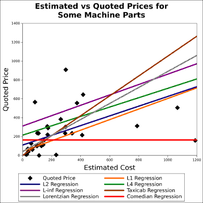
Estimated prices and quoted prices were collected for a sample of 36 machine parts. This data set is interesting because it has a definite overall trend, but contains several gross errors. This makes it useful to test the robustness of generalized orthogonal regressions. Seven types of regression were tested.
Machine learning is powerful because you don't have to understand how it works in order to use it. You don't have to understand the subject being studied either — although the practitioner should if possible. If not possible, he should defer to a better practitioner. In the present problem, the purpose really is not to say anything about yacht hulls, it is only to illustrate techniques for linear regression.
The test program YACHT calls the classical subroutines DHFTI, CHEB, and
L1 to compute the ℓ2, ℓ∞, and ℓ1 regressions.
Subroutine GORTH is then called to attempt to replicate these results.
Accuracy of the computed solution may be assessed with the coefficient of determination, defined as:
cd = 1 - ∑(yi - ŷi)² / ∑(yi - yave)²;This statistic lends itself to being modified to suit the ℓ1 and ℓ∞ metrics:
	cd1 = 1 - ∑|yi - ŷi| / ∑|yi - ymed|
     cd∞ = 1 - max(yi - ŷi) / ½(max(yi) - min(yi))
The GORTH ℓ2 result has the same coefficient of determination as DHFTI
up to machine precision. The GORTH ℓ1 result has the same coefficient of determination as
L1 up to 11 significant digits. The GORTH ℓ∞ result has a coefficient of
determination 0.3% less than that of CHEB.
Regressions are computed for the Lorentzian and Median residual criteria, and the Comedian, Lorentzian, ℓ1, and ℓ∞ isosceles criteria. As should be expected, the best coefficient of determination according to the ℓ1, ℓ2, and ℓ∞ norms was found by minimizing these residuals.

From the graph it appears that the Lorentzian criterion is lower order than ℓ1, and that the median criterion is lower still.
The isosceles criteria did not perform especially well on this problem. The isosceles-Lorentzian was quite similar to the ℓ2 result. The taxicab criterion was noticeably bad.

This well-known data set [Anderson, 1935] consists of 4 measurements each of 150 plant specimens, representing 3
species of iris. The 150×4 matrix was factored by algorithm PDQ according to the ℓ1,
ℓ2,, ℓ∞, and Lorentzian norms. The ℓ2 factorization is the singular
value decomposition; the other factorizations are analogues of the singular value decomposition. The first two columns
of the resulting matrix P were plotted.
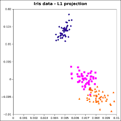

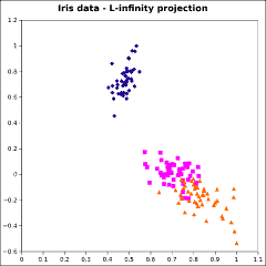
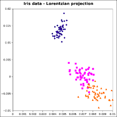
The graphs are not identical, but the differences are slight. It is not apparent that there is any advantage of
using one of these alternative factorizations instead of the SVD.
Program t_go solves a small artificial linear system by a scheme of factoring matrix A, then in turn solving the overdetermined and underdetermined sides of the problem, according to the ℓ2, ℓ1, ℓ∞, and Lorentzian norms and their corresponding isosceles orthogonality criteria. It produces the results:
 at begin, A is:
    2.000       -3.000       -1.000       -6.000       -2.000        0.000        5.000       -5.000
   -1.000        1.000        0.000        5.000        4.000       -1.000        3.000        2.000
    0.000        2.000        2.000        3.000        7.000       -4.000        2.000        2.000

 B is:
   -3.000        4.000        6.000       -1.000       -1.000
    2.000        2.000       -1.000        0.000        0.000
    0.000       -2.000        0.000        1.000        2.000

 Call gosolv with criterion: 2

 Solution X:
   -1.779        0.000      -0.1073E-02   0.1692E-02    0.000
  -0.7131E-05   0.1455E-03  -0.2394E-03   0.3388E-03    0.000
  -0.6376E-02   -2.247      -0.3310E-01   0.5405        1.000
  -0.7910E-02   0.6870E-01  -0.5134E-01  -0.9386E-05    0.000
  -0.5331E-04   0.5328E-03   0.3486      -0.3292E-01    0.000
   0.4114E-01  -0.3542       0.4314E-04  -0.4993E-04    0.000
   0.1007       0.4333       0.8089E-01  -0.1562E-01    0.000
  -0.5400E-07  -0.3287E-04   -1.191       0.8994E-01    0.000

 Call gosolv with criterion: T

 Solution X:
   -1.626       0.1074       0.7898E-01  -0.1406E-01    0.000
   0.6986E-02  -0.2407E-01  -0.3202E-01   0.5318E-02    0.000
  -0.1004E-01   -3.145       0.4602E-01   0.5829        1.000
   0.3411E-01  -0.1178      -0.1564       0.2596E-01    0.000
  -0.3366E-01   0.5994       0.1337      -0.2234E-01    0.000
   0.2920E-01  -0.1008      -0.1339       0.2223E-01    0.000
   0.1041       0.1292       0.2545      -0.2847E-01    0.000
   0.2401E-01  -0.8285E-01  -0.7697       0.2390E-01    0.000

 Call gosolv with criterion: S

 Solution X:
   0.4649E-02  -0.7797E-02  -0.6659E-02  -0.2578E-03    0.000
  -0.9296E-01   -1.790       -1.329       0.9056E-02    0.000
  -0.6749E-01  -0.1109E-01   0.1383        0.000        0.000
   0.6018        1.097       0.4295E-01    0.000        0.000
  -0.2022       0.2533E-01   0.4417E-01    0.000        0.000
  -0.3019E-03   0.5061E-03  -0.6873      -0.2849      -0.6000
  -0.3253E-01   0.6059E-01   0.4958E-01  -0.1366      -0.2000
  -0.2686E-02  -0.9932      -0.4526       0.5784E-01    0.000

 Call gosolv with criterion: R

 Solution X:
  -0.2310E-01  -0.9739       0.1212        0.000       0.4919
   0.9348E-02  -0.4316      -0.6656       0.2311       0.7251
   -1.141      -0.9810       0.7040E-01   0.3141       0.1186E-01
   0.4742E-01   0.1531      -0.2576      -0.2926E-01  -0.6250E-01
   0.1508       0.4928E-01   0.1809      -0.8519E-07   0.3152E-01
   0.3612E-01    0.000      -0.1961      -0.1621E-01  -0.1630
  -0.4572E-01   0.4741       0.2428      -0.3366E-01  -0.5064E-01
   0.6503      -0.4637      -0.2867        0.000      -0.2895E-01
This shows that for an underdetermined system, widely different answers are possible. Solution by generalized
orthogonality offers a distinct approach.
Generalized orthogonality seems to be mostly of theoretical mathematical interest. Package GOPAK is
able to compute these vectors using standard optimization techniques for some small problems. High computational
expense and numerical difficulties are prohibitive for larger problems.
It has not been shown that there is a compelling practical reason to prefer these generalized methods over traditional linear algebra. They are offered as curiosities, with the hope that a use for them remains to be discovered.
Formula for Gram-Schmidt orthogonalization
	Given vectors u and v, seek a scalar c such that u and (v-cu) are orthogonal.

     u · (v-cu) = 0
     ∑(uivi - cui²) = 0
     c = ∑uivi / ∑ui²
     c = u·v / u·u

This also minimizes the length of v-cu, because:

     ℓ² = ∑(vi-cui)²

Differentiate with respect to c and set equal to zero:

     dℓ²/dc = 2 ∑(vi-cui)(-ui) = 0
     ∑(-uivi + cui²) = 0
     c = u·v / u·u
Expanding absolute value bars
The composite function f(g(x)) = |g(x)| may be written:

     |g(x)| = {-g(x), g(x) < 0}
              {0,     g(x) = 0}
              {+g(x), g(x) > 0}

Its derivative df/dx = (df/dg)(dg/dx) is then:

     df/dx = {-dg/dx,    g(x) < 0}
             {+dg/dx,    g(x) > 0}
             {undefined, g(x) = 0}

For present purposes, the derivative at zero shall be treated as zero,
as this is the average of the value on either side.
A common approximation of the absolute value
     a = |u| ≈ (u² + τ)½
     da/dx ≈ (u / (u² + τ)½) du/dx
where τ is very small.
Differentiable approximation for a quantile of a data set
Given an array wi, 1...i...n, any quantile wq must
satisfy the counting function:

     ∑{-1, wi < wq} = (1 - q)n - qn
      {+1, wi > wq}

Using the approximation of the absolute value, this may be written:

     ∑(wi - wq) / ((wi - wq)² + τ)½ = (1 - 2q)n

Differentiating with w as a function of x shows that:

∂wq/∂x ≈ (∑ ∂wi/∂x ((wi - wq)² + τ)-3/2) / (∑ ((wi - wq)² + τ)-3/2)
Smooth approximation to the maximum and its derivative (Birbil et. al., 2003)
Define the function f(a,b) = ½(a + b + ((a-b)² + τ)½)
where τ is very small.  Then,

     max(w1, w2, ... wi ... wn) ≈
     h = f(f(...f(...f(0, w1), w2), ..., wi), ..., wn)

Let f(i) denote the approximate maximum of the first i elements of w.  Then,

     ∂h/∂x = ∂f(n)/∂wn ∂wn/∂x + ...
        + ∂f(i+1)/∂f(i)(∂f(i)/∂wi ∂wi/∂x + ...
          + ∂f(2)/∂f(1)(∂f(1)/∂w1 ∂w1/∂x))

Now let p(a,b) = ∂f/∂a = ½(1 + (a-b)/((a-b)² + τ)½)
        q(a,b) = ∂f/∂b = ½(1 - (a-b)/((a-b)² + τ)½)

Observe that while f is symmetric with respect to a and b, its derivatives are not.
The approximate derivative of the maximum may be written:

     ∂h/∂x = q(f(n-1),wn) ∂wn/∂x + p(f(n-1),wn)(q(f(n-2),wn-1) ∂wn-1/∂x + ...
       + p(f(i),wi+1)(q(f(i-1),wi) ∂wi/∂x + ...
         + p(f(1),w2)(q(0,w1) ∂w1/∂x) ...) ...)
Comedian orthogonality existence and uniqueness
Given vectors u and v, seek a scalar c such that:

     com(u, (v-cu)) = 0
     med(ui(vi-cui)) = 0

Define the function

     f(c) = med(uivi - cui²)

Each component of the resultant vector is continuous with respect to c.
Let the components be written in ascending order.  In response to a change in
c, for the component in median position in this ordering to change places
with its adjacent component, umvm - cum² = um+1vm+1 - cum+1²,
because they are continuous.  Therefore, f(c) is continuous.

    df/dc = -um² ≤ 0, so f(c) is decreasing.

For a sufficiently large negative c, f(c) = med(uivi - cui²) > 0
For a sufficiently large positive c, f(c) = med(uibi - cui²) < 0

f(c) is continuous, monotonic, and has values less than and greater than zero.
Therefore the equation f(c) = 0 has a solution, either at a unique point
or a single interval.
Algorithm to minimize the ℓ1 length of a linear combination of two vectors
Given vectors u and v, seek a scalar c to minimize:

     ℓ1 = ∑|vi - cui|

     ∑|vi - cui| = ∑ { vi - cui, vi - cui > 0}
                     {-vi + cui, vi - cui < 0}

Differentiate with respect to c and set equal to zero:

     dℓ/dc = ∑{-ui, vi - cui > 0} = ∑ {-ui, {c < vi/ui, ui > 0}} = 0
              { ui, vi - cui < 0}     {     {c > vi/ui, ui < 0}}
                                      { ui, {c > vi/ui, ui > 0}}
                                      {     {c < vi/ui, ui < 0}}

Combining cases:

    ∑{-|ui|, c < vi/ui} = 0
     {0,     c = vi/ui}
     {+|ui|, c > vi/ui}


Thus, c must be chosen so that the sum of absolute values of ui for
terms satisfying c > vi/ui must equal the sum of absolute values
of ui for terms for which c < vi/ui.

begin
Compute ½∑|ui|
Compute vi/ui for all i and sort.
Accumulate total t, adding each term |ui| in order of ascending vi/ui
When tj ≥ ½∑|ui| at some step j, return c = vj/uj
ℓ1 Isosceles orthogonality against n vectors
Given a vector of m components vi, and n vectors of m components uij,
seek factors x and y, such that the linear combination  v' = yvi - ∑xluil
satisfies the conditions

     fj = v' ⋄ uj = 0
     v' ⋄ uj = ½∑(|yvi - ∑xluil + uij| - |yvi - ∑xluil - uij|)

To solve this system of equations numerically, use the Jacobian matrix:


     ∂fj/∂xk = ∑{+uik, +uij < vi' < -uij}
                {-uik, -uij < vi' < +uij}
                {0, otherwise          }

     ∂fj/∂y = ∑{-vi, +uij < vi' < -uij}
               {+vi, -uij < vi' < +uij}
               {0, otherwise         }

Because ℓ1 Isosceles orthogonality is not homogeneous, that is, u ⊥ v ⇏ u ⊥ av
in general for a scalar a, require also unit length of v'
For the ℓ1 norm, this gives:

     f0 = ∑|vi'| - 1 = ∑|yvi - ∑xluil| - 1 = 0

     ∂f0/∂xk = ∑{+uik, vi' < 0}
                {0,    vi' = 0}
                {+uik, vi' > 0}

     ∂f0/∂y = ∑{-vi, vi' < 0}
               {0,   vi' = 0}
               {+vi, vi' > 0}
Relationship of ℓ1 geometry and fuzzy logic
Interestingly, the taxicab-isosceles formula can be obtained by the use
of fuzzy logic. The standard intersection operator in fuzzy logic is
the minimum.  The standard union operator in fuzzy logic is the maximum.
To obtain the codeviation, begin with an expression for logical equivalence:

     u ⇔ v = (u ∧ v) ∨ (¬u ∧ ¬v)
     max(min(u, v), min(1-u, 1-v))

In switching from logical variables to scalar variables, the effects of the
min and max operations are unchanged. For negation, values must be
reflected across 0 instead of ½, thus ¬u becomes -u rather than 1-u,
resulting in:

     u ⇔ v = max(min(u, v), min(-u, -v))

Compare the expression derived from geometry with the expression derived
from fuzzy logic; they are identical.

     ½(|u+v| - |u-v|) ≡ max(min(u, v), min(-u, -v))

This demonstrates a remarkable relationship between fuzzy logic and ℓ1
geometry. Two distinct approaches have led to the same formula.
For the purposes of computation, the min/max formula is to be
preferred, since it is not susceptible to subtractive cancellation.
ℓ∞ Isosceles orthogonality against n vectors
Given a vector of m components vi, and n vectors of m components uij,
seek factors x and y, such that the linear combination  v' = yvi - ∑xluil
satisfies the condition

     fj = v' ▫ uj = 0
     v' ▫ uj = ½(max|yvi - ∑xluil + uij| - max|yvi - ∑xluil - uij|) = 0

To solve this system of equations numerically, use the Jacobian matrix:

∂fj/∂xk = ½({+upk, vp' + upj < 0} - {+uqk, vq' - uqj < 0})
            {0,    vp' + upj = 0}   {0,   vq' - uqj = 0}
            {-upk, vp' + upj > 0}   {-uqk, vq' - uqj > 0}

∂fj/∂y = ½({-vp, vp' + upj < 0} - {-vq, vq' - uqj < 0})
           {0,   vp' + upj = 0}   {0,   vq' - uqj = 0}
           {+vp, vp' + upj > 0}   {+vq, vq' - uqj > 0}

where p is the index of the maximum element of |v' + uj|
and q is the index of the maximum element of |v' - uj|

Because ℓ∞ Isosceles orthogonality is not homogeneous, require unit length of v'

     f0 = max|vi'| - 1 = max|yvi - ∑xluil| - 1 = 0

     ∂f0/∂xk = {+urk, vr' < 0}
               {0,    vr' = 0}
               {-urk, vr' > 0}

     ∂f0/∂y = {-vr, vr' < 0}
              {0,   vr' = 0}
              {+vr, vr' > 0}

where r is the index of the maximum element of |v'|
Lorentzian-Isosceles orthogonality against n vectors
Given a vector of m components vi, and n vectors of m components uij,
seek factors x and y, such that the linear combination  v' = yvi - ∑xluil
satisfies the condition

     fj = ∑log(1 + |v' + uj|) - log(1 + |v' - uj|) = 0

To solve this system of equations numerically, use the Jacobian matrix:

∂fj/∂xk = ∑({+1/(1 - vi' - uij), vi'+uij < 0} - {+1/(1 - vi' + uij), vi'-uij < 0}) uik
            {0,                 vi'+uij = 0}    {0,                 vi'-uij = 0}
            {-1/(1 + vi' + uij), vi'+uij > 0}   {-1/(1 + vi' - uij), vi'-uij > 0}

∂fj/∂y = ∑({+1/(1 - vi' - uij), vi'+uij < 0} - {+1/(1 - vi' + uij), vi'-uij < 0}) (-vi)
           {0,                 vi'+uij = 0}    {0,                 vi'-uij = 0}
           {-1/(1 + vi' + uij), vi'+uij > 0}   {-1/(1 + vi' - uij), vi'-uij > 0}


Because Lorentzian-Isosceles orthogonality is not homogeneous, require unit length of v'

     f0 = ∑log(1+|vi'|) - 1 = 0

     ∂f0/∂xk = ∑{+uik/(1-vi'), vi' < 0}
                {0,           vi' = 0}
                {-uik/(1+vi'), vi' > 0}

     ∂f0/∂y = ∑{-vi/(1-vi'), vi' < 0}
               {0,           vi' = 0}
               {+vi/(1+vi'), vi' > 0}
Comedian orthogonality against n vectors
Given a vector of m components vi, and n vectors of m components uij,
seek factors x, such that the linear combination v' = vi - ∑xluil
satisfies the condition

     fj = com(v', uj) = 0
     fj = med((vi - ∑xluil)uij) = 0
     fj = uoj(vo - ∑xluol) = 0

where o is the index of the median.  To solve this system of equations numerically,
use the Jacobian matrix:

     ∂fj/∂xk = -uojuok
Euclidean orthogonality against n vectors
Given a vector of m components vi, and n vectors of m components uij,
seek factors x, such that the linear combination  v' = vi - ∑xkuik
satisfies the condition

     uj · v' = 0
     uj·vi - ∑uj·xkuk = 0
     ∑∑uijuikxk = ∑uijvi
     UTUx = UTv
     x = U+v

Which may be recognized as the normal equations for the least-squares
solution of the linear system.  Alternatively, solve the system numerically
using the Jacobian matrix:

     ∂fj/∂xk = -∑uijuik
ℓ1 residual orthogonality against n vectors
Given a vector of m components vi, and n vectors of m components uik,
seek factors x, such that the linear combination v' = vi - ∑xkuik
has minimum ℓ1 norm.

     f = ∑|vi'| = ∑|vi - ∑xkuik|

To minimize this function numerically, use the gradient:

     ∂f/∂xk = ∑{+uik, vi' < 0}
               {0,    vi' = 0}
               {-uik, vi' > 0}
ℓ∞ residual orthogonality against n vectors
Given a vector of m components vi, and n vectors of m components uik,
seek factors x, such that the linear combination v' = vi - ∑xkuik
has minimum ℓ∞ norm.

     f = max|vi'| = max|vi - ∑xkuik|

To minimize this function numerically, use the gradient:

     ∂f/∂xk = {+urk, vr' < 0}
              {0,    vr' = 0}
              {-urk, vr' > 0}

where r is the index of the maximum element of |v'|
Lorentzian residual orthogonality against n vectors
Given a vector of m components vi, and n vectors of m components uik,
seek factors x, such that the linear combination v' = vi - ∑xluil
has minimum Lorentzian norm.

     f = ∑log(1 + |vi'|) = ∑log(1 + |vi - ∑xluil|)

To minimize this function numerically, use the gradient:

     ∂f/∂xk = ∑{+uik/(1-vi'), vi' < 0}
               {0,           vi' = 0}
               {-uik/(1+vi'), vi' > 0}
Median absolute residual orthogonality against n vectors
Given a vector of m components vi, and n vectors of m components uik,
seek factors x, such that the linear combination v' = vi - ∑xluil
has minimum median absolute value.

     f = med(|vi'|) = med(|vi - ∑xluil|)

To minimize this function numerically, use the gradient.

     ∂f/∂xk = {+uok, vo' < 0}
              {0,    vo' = 0}
              {-uok, vo' > 0}

where o is the index of the median element of the array |vi-∑xluil|